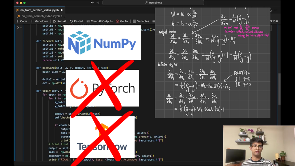
Neural networks have revolutionized the field of artificial intelligence, enabling complex problem-solving and learning from vast amounts of data. In this article, we will explore how to create a neural network from scratch using only Python and NumPy, without relying on frameworks like PyTorch or TensorFlow, achieving an accuracy of 97.56%! This approach will give you a deeper understanding of the fundamentals of neural networks and their mathematical underpinnings.
YouTube Video: https://youtu.be/Iz69t6HOC3c?si=MDQbLb7wxq3J74F2
Full Code: https://github.com/Lumos-Academy/educational/blob/main/neural-nets/nn_from_scratch.ipynb
Understanding the Dataset
To begin, we need to discuss the dataset we will be using, known as the Digit Recognizer dataset from Kaggle. This dataset is a classic in the field of computer vision and consists of images of handwritten digits ranging from 0 to 9.
The training set contains 42,000 images, each represented as a 28×28 pixel grid, which totals 784 pixels. Each image is flattened into a single row of 784 pixel values. The first column of the dataset contains the labels corresponding to each digit, while the subsequent columns represent the pixel values. The pixel values range from 0 (black) to 255 (white).
Data Input and Output
Our goal is to train a neural network that takes these pixel values as input and predicts the corresponding digit label. We will compare the predicted labels with the actual labels to calculate the error rate, known as loss, which will guide the training process. This iterative process allows the neural network to improve its predictions over time.
What is a Neural Network?
A neural network is composed of interconnected layers of nodes, or neurons, which are modeled after the human brain. The primary components of a neural network include:
Input Layer: This layer receives the input data, in our case, the pixel values from the images.
Hidden Layers: These layers perform computations on the inputs, extracting features and learning representations.
Output Layer: This layer produces the final output, which corresponds to the predicted digit.
Each connection between neurons has an associated weight, which is adjusted during training to minimize the prediction error. Additionally, each neuron has a bias that helps to fine-tune the output of the neuron.
Neurons and Perceptrons
Each neuron in the network performs a simple computation: it takes input values, multiplies them by their corresponding weights, adds the bias, and then applies an activation function. The activation function introduces non-linearity into the model, enabling it to learn complex patterns in the data.
Activation Functions
Activation functions play a crucial role in neural networks by determining whether a neuron should be activated or not based on the input it receives. Some commonly used activation functions include:
ReLU (Rectified Linear Unit): Outputs the input directly if it is positive; otherwise, it outputs zero.
Sigmoid: Outputs a value between 0 and 1, often used for binary classification.
Softmax: Converts the outputs of a neural network into probabilities, typically used in the output layer for multi-class classification.
For our digit recognition task, we will use the Softmax activation function in the output layer to produce a probability distribution over the 10 possible digit classes (0-9).
Mathematical Foundations
Understanding the mathematics behind neural networks is essential for grasping how they function. The key mathematical operations include:
Dot Product: This operation is used to compute the weighted sum of inputs. For two vectors, the dot product is the sum of the products of their corresponding entries.
Gradient Descent: This optimization algorithm is used to minimize the loss function by iteratively updating the weights and biases based on the gradients.
Training the Neural Network
The training process of a neural network involves two main steps: the forward pass and the backward pass. During the forward pass, the input data is fed through the network to produce an output. The backward pass involves calculating the gradients of the loss function with respect to the weights and biases and updating them accordingly.
Forward Pass
In the forward pass, we compute the output of each layer using the current weights and biases. The process is as follows:
- Hidden Layer Computation:
- Calculate the weighted sum of inputs for each neuron in the hidden layer.
- Apply the activation function (e.g., ReLU) to obtain the output of the hidden layer.
- Output Layer Computation:
- Calculate the weighted sum of hidden layer outputs for the output layer neurons.
- Apply the Softmax function to obtain the predicted probabilities for each class.
Backward Pass
During the backward pass, we compute the gradients of the loss function with respect to the weights and biases. The steps include:
- Loss Computation:
- Compute the loss using the predicted output (from the Softmax function) and the actual labels (using a loss function like cross-entropy).
- Output Layer Gradients:
- Calculate the gradient of the loss with respect to the output layer activations (before Softmax).
- Use these gradients to calculate the gradient with respect to the output layer weights and biases.
- Hidden Layer Gradients:
- Backpropagate the gradients to the hidden layer by calculating the gradient with respect to the hidden layer activations (before ReLU).
- Use these gradients to calculate the gradient with respect to the hidden layer weights and biases.
- Parameter Update:
- Update the weights and biases using the gradients and a learning rate (using an optimization algorithm like stochastic gradient descent).
Implementing the Neural Network in Code
Now that we have a solid understanding of the concepts and mathematics, we can move on to the implementation of our neural network using Python and NumPy.
Data Preparation
First, we need to load our dataset and split it into training and testing sets. We will also normalize the pixel values to be between 0 and 1 for better performance during training.
import numpy as np

import pandas as pd

# Load the dataset

data = pd.read_csv('data.csv')

# Split the dataset into training and testing sets

train_data = data.iloc[:33600]

test_data = data.iloc[33600:]

# Normalize pixel values

X_train = train_data.iloc[:, 1:].values / 255.0

y_train = train_data.iloc[:, 0].values

X_test = test_data.iloc[:, 1:].values / 255.0

y_test = test_data.iloc[:, 0].values

# One Hot Encode

y_train_encoded = np.eye(10)[y_train]

y_test_encoded = np.eye(10)[y_test]
Neural Network Initialization
Next, we will create a neural network class that initializes the weights and biases and contains methods for training and predicting.
class NeuralNetwork:

    def __init__(self, input_size, hidden_size, output_size):

        self.input_size = input_size

        self.hidden_size = hidden_size

        self.output_size = output_size

        self.W1 = np.random.randn(self.input_size, self.hidden_size) * np.sqrt(2/self.input_size)

        self.b1 = np.zeros((1, self.hidden_size))

        self.W2 = np.random.randn(self.hidden_size, self.output_size) * np.sqrt(2/self.hidden_size)

        self.b2 = np.zeros((1, self.output_size))
Neural Network Forward Pass
Now to get outputs from inputs, we have to implement the forward method within the NeuralNetwork class.
def forward(self, X):

        self.z1 = np.dot(X, self.W1) + self.b1

        self.a1 = relu(self.z1)

        self.z2 = np.dot(self.a1, self.W2) + self.b2

        self.a2 = softmax(self.z2)

        return self.a2
Neural Network Backward Pass
For our network to learn, and tune our weights and biases parameters to become more accurate representations, we need to implement the backward pass.
def backward(self, X, y, output, learning_rate):

        batch_size = X.shape[0]

        delta2 = output - y

        dW2 = np.dot(self.a1.T, delta2) / batch_size

        db2 = np.sum(delta2, axis=0, keepdims=True) / batch_size

        delta1 = np.dot(delta2, self.W2.T) * relu_derivative(self.a1)

        dW1 = np.dot(X.T, delta1) / batch_size

        db1 = np.sum(delta1, axis=0, keepdims=True) / batch_size

        # Update weights and biases

        self.W2 -= learning_rate * dW2

        self.b2 -= learning_rate * db2

        self.W1 -= learning_rate * dW1

        self.b1 -= learning_rate * db1
ReLU and Softmax
If you’re following along, you may have noticed that we haven’t implemented relu, relu_derivative, or softmax, so let’s do that now.
def relu(x):

    return np.maximum(0, x)

def relu_derivative(x):

    return np.where(x>0, 1, 0)

def softmax(x):

    exp_x = np.exp(x - np.max(x, axis=1, keepdims=True))

    return exp_x / np.sum(exp_x, axis=1, keepdims=True)
Training Method
The training method will utilize the forward and backward passes, updating weights and biases based on the calculated gradients. It will also print the loss and accuracy of every tenth epoch.
def train(self, X, y, epochs, learning_rate, batch_size):

        for epoch in range(epochs):

            for i in range(0, X.shape[0], batch_size):

                X_batch = X[i:i+batch_size]

                y_batch = y[i:i+batch_size]

                output = self.forward(X_batch)

                self.backward(X_batch, y_batch, output, learning_rate)

            if epoch % 10 == 0:

                output = self.forward(X)

                loss = -np.mean(np.sum(y * np.log(output + 1e-8), axis=1))

                accuracy = np.mean(np.argmax(output, axis=1) == np.argmax(y, axis=1))

                print(f"Epoch {epoch}, Loss: {loss:.4f}, Accuracy: {accuracy:.4f}")

        # Print final results

        output = self.forward(X)

        loss = -np.mean(np.sum(y * np.log(output + 1e-8), axis=1))

        accuracy = np.mean(np.argmax(output, axis=1) == np.argmax(y, axis=1))

        print(f"FINAL | Epoch {epoch}, Loss: {loss:.4f}, Accuracy: {accuracy:.4f}")
Prediction Method
Finally, we will implement a very simple method for making predictions based on new input data.
def predict(self, X):

        """Make predictions on new data"""

        return self.forward(X)
Evaluating the Model
After training our neural network, we will evaluate its performance on the test set to see how well it generalizes to unseen data. We will calculate the accuracy by comparing the predicted labels with the actual labels.
input_size = 784

hidden_size = 128

output_size = 10

nn = NeuralNetwork(input_size, hidden_size, output_size)

nn.train(X_train, y_train_encoded, epochs=50, learning_rate=0.1, batch_size=32)

# Evaluate accuracy on the test set

predictions = nn.predict(X_test)

predicted_labels = np.argmax(predictions, axis=1)

accuracy = np.mean(predicted_labels == y_test)

print(f"Test accuracy: {accuracy:.4f}")
If you seed your program with NumPy, you should see a 97.56% accuracy, which is really good!
np.random.seed(42) # Set random seed for reproducibilityConclusion
In this article, we successfully created a neural network from scratch using Python and NumPy. We explored the fundamental concepts, mathematical operations, and the implementation process. This hands-on approach allows for a deeper understanding of how neural networks function and how they can be applied to real-world problems.
Neural networks are powerful tools in artificial intelligence, and mastering their principles is essential for anyone interested in the field. We hope this guide provides a solid foundation for your journey into neural networks and machine learning.