Neural networks are a really big deal in the fields of artificial intelligence and machine learning. Among the many applications of these networks, one of the most foundational and widely recognized is the task of digit recognition.
This tutorial aims to go through the process of building a digit recognizer using a neural network, by providing a comprehensive, line-by-line explanation of the code involved. We’ll delve into the MNIST dataset, a common benchmark in the field, which consists of 70,000 images of handwritten digits. By the end of this article, you’ll have a thorough understanding of how to construct, train, and evaluate a neural network designed to recognize these digits with impressive accuracy.
Each segment of the code will be meticulously explained, ensuring that you grasp not just the ‘how’ but also the ‘why’ behind each step. Whether you’re coding along or simply seeking to deepen your theoretical knowledge, this tutorial is structured to enhance your understanding of neural networks in a clear and methodical manner.
Imports
The first thing we’ll need to do is import the necessary dependencies, which are the third-party libraries of code we’ll need to create our neural network.
import numpy as np
import torch
import torch.nn as nn
import torch.optim as optim
import pandas as pd
import matplotlib.pyplot as plt
Reproducibility
Setting random seeds for reproducibility is an essential practice in machine learning and neural network training. Random processes such as weight initialization, data shuffling, and dropout can lead to variations in results each time a model is trained. To ensure consistent outcomes, random seeds are set, which fix the sequence of random numbers generated by the algorithm. This means that every time the code is run, these random processes will produce the same results, allowing for exact replication of experiments.
Reproducibility is crucial for debugging, comparing model performance, and sharing results with others. By setting a random seed, you make your experiments reliable and verifiable, as others can run your code and obtain the same results. In Python, setting a random seed is straightforward with libraries like NumPy, TensorFlow, and PyTorch.
seed = 42
np.random.seed(seed)
torch.manual_seed(seed)
if torch.cuda.is_available():
    torch.cuda.manual_seed(seed)
    torch.cuda.manual_seed_all(seed)  # if you are using multi-GPU.
torch.backends.cudnn.deterministic = True
torch.backends.cudnn.benchmark = False
Loading and Preparing Data
Data from Kaggle: https://www.kaggle.com/competitions/digit-recognizer/data
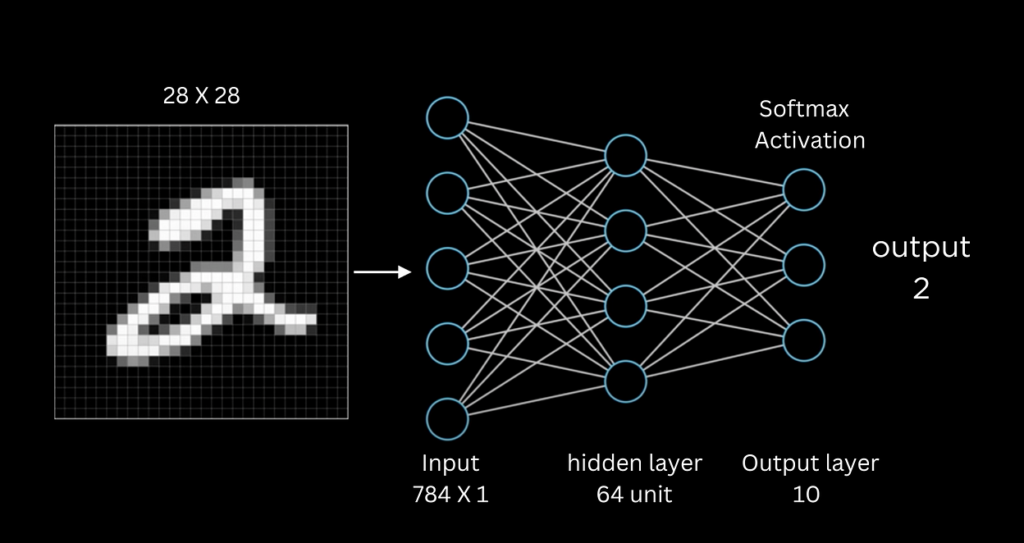
The data consists of 70,000 28-pixel-by-28-pixel images of grayscale handwritten digits. The 70,000 images are broken into a training set of 42,000 images which we will be loading, and a 28,000 image test set that we will deal with later.
The data is formatted as a csv with a label column which tells us the digit that each image represents, and 784 columns (28*28 = 784), each with a pixel value between 0 (black) and 255 (white).

Though the data can be visualized here as a spreadsheet, it is actually a .csv file where each number is delimited, or separated by commas.
To load the data, we’ll use numpy to load the csv file:
dataset = np.loadtxt('data/train.csv', delimiter=',', skiprows=1)We get the dataset from train.csv in our data folder, which, again, delimits each data point with commas, and we skip the first row which contains the names of each of the columns, ‘label’, ‘pixel0’…’pixel783’.
Then, we split the train set into X and y. X is the independent variable, which is the pixel values themselves, and y is the dependent variable which contains the labels (which depend on the pixel values).
We get X (the pixel values) from every column except the first one:
X = dataset[:,1:]And we extract y (the label) from the first column:
y = dataset[:, 0]The next detail is very important; we need to normalize our data. The pixel values are between 0 and 255, but it helps a lot to squeeze the values to be within a smaller range, specifically between 0 and 1.
The benefit of normalizing the input data is that it avoids large values in the internal computations of the neural network which could make the training process difficult.
It’s pretty simple, all we have to do is:
X = X / 255.0After this, we have to make the data compatible with PyTorch by converting it into tensors of specific types.
X = torch.tensor(X, dtype=torch.float32)
y = torch.tensor(y, dtype=torch.int64)
Now that we’re done with loading and preparing the data, we’re going to get into the really juicy part of deep learning.
Let’s create our model.
model = nn.Sequential(
    nn.Linear(784, 300),
    nn.ReLU(),
    nn.Linear(300, 300),
    nn.ReLU(),
    nn.Linear(300, 10)
)
The first layer needs to have 784 neurons as input, since there are 784 values in X, one for each pixel. The final layer needs to have 10 neurons as output since we are predicting out of 10 digits between 0 and 9.
Other than that, the neuron values of hidden layers are kind of arbitrary, but there are some rules of thumb to decide how many neurons to have in each layer.
Jeff Heaton suggests in Introduction to Neural Networks for Java (second edition):
- The number of hidden neurons should be between the size of the input layer and the size of the output layer.
- The number of hidden neurons should be 2/3 the size of the input layer, plus the size of the output layer.
- The number of hidden neurons should be less than twice the size of the input layer.
What is ReLU?
Each neuron in the network needs an activation function. How much should a neuron “activate” based on its internal calculation of the input*weight+bias?
There are a variety of activation functions but this is what ReLU looks like, graphed.
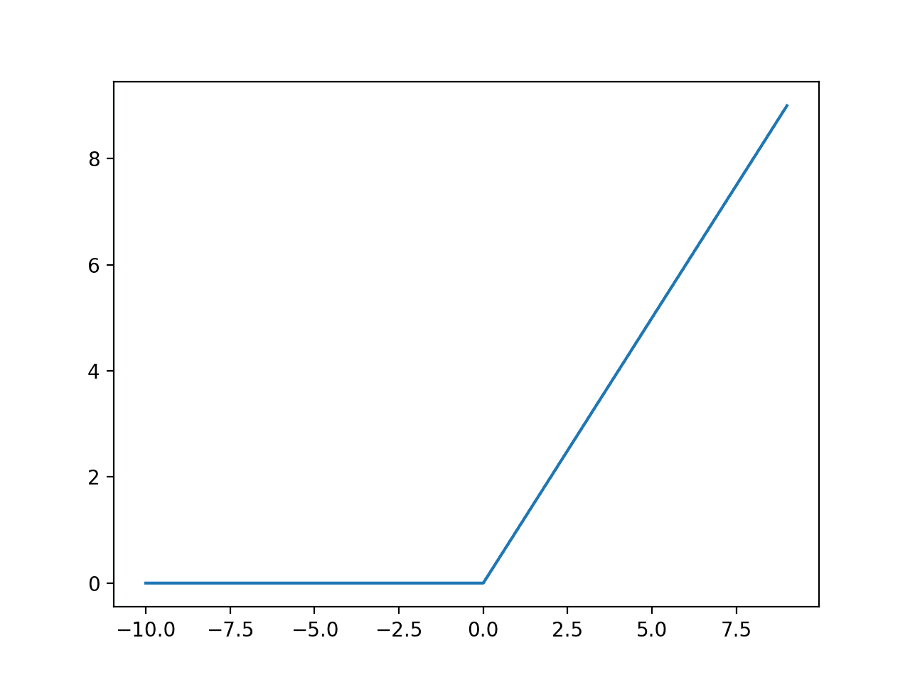
If the value of the input*weight+bias is less than 0, the output of the neuron will be 0, it won’t “activate”. If the value is greater than 0, it will output whatever the input was (y=x).
Loss Function and Optimizers
A loss function, also known as the error function, quantifies how well a single prediction of the algorithm is compared to the actual target value.
An optimizer is a function or an algorithm that adjusts the attributes of the neural network, such as weights and learning rates, to reduce the loss and improve the accuracy.
Here’s how we code it out:
loss_fn = nn.CrossEntropyLoss()  # binary cross entropy
optimizer = optim.Adam(model.parameters(), lr=0.001)
We’re using a specific loss function, called the cross entropy loss and a specific optimizer called Adam.
We’re also specifying the learning rate of the optimizer, which controls how much to change the model in response to the estimated error each time the model weights are updated. We set it at 0.001, but you can generally experiment with values less than 1.0 and greater than 10^-6. I typically move between 0.1, 0.01, and 0.001. Too fast, and your model will overshoot, change the model too much, and may get worse performance. Too slow, and your model won’t learn fast enough.
Training Loop
We now need to implement a training loop for a neural network over 10 epochs with a batch size of 10. In each epoch, the dataset is divided into smaller batches, and for each batch, a forward pass is performed to predict the outputs using the model.
The loss between the predicted and actual labels is then computed using our predefined Cross Entropy Loss function.
Gradients are measures of how much the loss changes with respect to each model parameter (weights and biases). They guide the adjustments needed to minimize the loss and improve the model’s predictions during training.
After computing the loss, the gradients are reset to zero, backpropagation is performed to compute the gradients of the loss with respect to the model parameters, and the Adam optimizer updates the model parameters based on these gradients.
# Run the training loop
n_epochs = 10
batch_size = 10

for epoch in range(n_epochs):
    for i in range(0, len(X), batch_size):
        Xbatch = X[i:i + batch_size]
        ybatch = y[i:i + batch_size]

        # Forward pass
        y_pred = model(Xbatch)

        # Compute loss
        loss = loss_fn(y_pred, ybatch)

        # Backward pass and optimization
        optimizer.zero_grad()
        loss.backward()
        optimizer.step()

    print(f'Finished epoch {epoch}, latest loss {loss.item()}')
Evaluate the Model
We evaluate a neural network model by first disabling gradient calculations to conserve resources.
Our code then makes predictions on the input data X and converts these predictions into class labels using the torch.argmax function. We need the torch.argmax function because the predictions will be a list of output values of each neuron, but we only need the neuron that activated the most to get the predicted class.
By comparing these predicted labels with the true labels y, the code calculates the accuracy of the model, which is the proportion of correct predictions.
with torch.no_grad():
    y_pred = model(X)
    predictions = torch.argmax(y_pred, dim=1)
    accuracy = (predictions == y).float().mean()
    print(f"Accuracy: {accuracy.item()}")
Make Predictions
We finally need to apply our model to make predictions on the test set.
# Load the test dataset
test_data_path = 'data/test.csv'
test_df = pd.read_csv(test_data_path)

# Prepare the test data
test_X = test_df.values
test_X = test_X / 255.0  # Normalize pixel values to [0, 1]
test_X = torch.tensor(test_X, dtype=torch.float32)

model.eval()

# Make predictions
with torch.no_grad():
    outputs = model(test_X)
    test_predictions = torch.argmax(outputs, dim=1).numpy()

# Create a DataFrame with ImageId and Label
image_ids = np.arange(1, len(test_predictions) + 1)  # Assuming ImageId starts from 1
submission_df = pd.DataFrame({
    'ImageId': image_ids,
    'Label': test_predictions
})

# Save to CSV file
submission_df.to_csv('submission.csv', index=False)
We load our dataset, normalize the pixel values like we did for the X of the training set, convert the model to evaluation mode, then make predictions on the test set, create a pandas DataFrame with the image id and predicted label, and save the DataFrame to a csv file.
And that’s all she wrote, folks! Leave a comment if you have any questions and like if you appreciated this content!
B.T.W. this simple neural network boasts an impressive 0.975 accuracy on the test set.
Full Code: https://github.com/Pursuit-Labs/neural-networks/blob/main/mnist/mnist.ipynb