
Hey everyone! We’re going to explore one of the most influential and powerful tools in the world of deep learning: Convolutional Neural Networks, or CNNs.
Convolutional Neural Networks have revolutionized many fields, particularly computer vision, due to their unparalleled ability to process and analyze visual data. They are the driving force behind advanced technologies like facial recognition systems, self-driving cars, and diagnostic tools in healthcare. The importance and impact of CNNs stem from their exceptional performance in recognizing patterns, shapes, and structures in images, making them invaluable for tasks involving large-scale visual data.
ConvNets are quite similar to traditional Neural Networks.
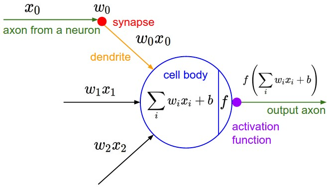
They consist of neurons with learnable weights and biases, where each neuron takes some inputs, computes a dot product, and optionally follows it with a non-linearity, an activation function. The entire network still represents a single differentiable score function, transforming raw image pixels at the input layer into class scores at the output layer. Additionally, CNNs have a loss function, like Softmax, on the last (fully connected) layer, and all the optimization techniques and learning strategies for regular Neural Networks apply to CNNs as well.
So, what’s different? CNN architectures make the explicit assumption that the input is an image, allowing us to encode specific properties into the architecture. This assumption makes the forward function more efficient and significantly reduces the number of parameters in the network.
In this post, we’ll be going over:
Architecture Overview ( An overview of the ConvNet architecture )
ConvNet Layers
ConvNet Architectures
Visualizing What ConvNets Learn
Transfer Learning
Architecture Overview
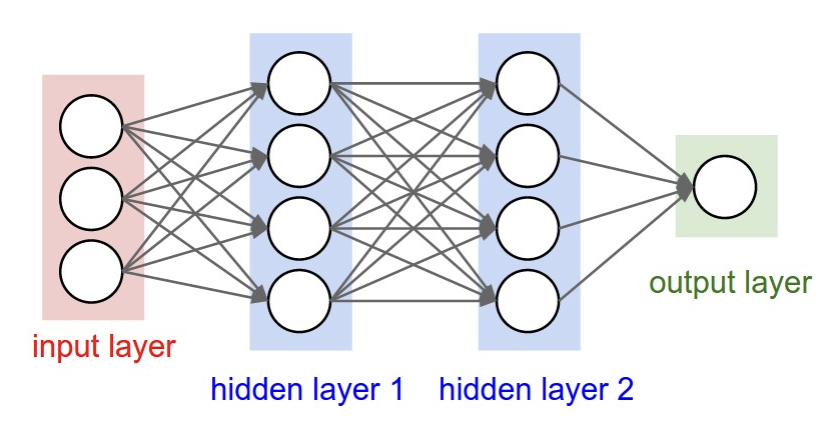
Recall: Regular Neural Nets. Neural Networks receive an input (a single vector) and transform it through a series of hidden layers. Each hidden layer is composed of neurons that are fully connected to all neurons in the previous layer, functioning independently without sharing any connections. The last fully-connected layer, called the “output layer,” represents the class scores in classification tasks.
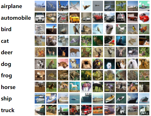
However, regular Neural Nets don’t scale well to full images. For example, in CIFAR-10, images are 32x32x3 (32 wide, 32 high, 3 color channels), so a single fully-connected neuron in a first hidden layer of a regular Neural Network would have 32*32*3 = 3072 weights. This might seem manageable, but as we move to larger images, such as 200x200x3, each neuron would require 200*200*3 = 120,000 weights. With multiple neurons, the number of parameters quickly becomes impractical, leading to inefficiency and overfitting.
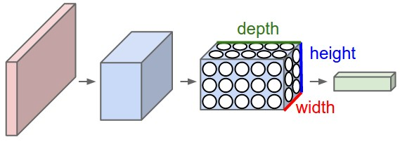
Convolutional Neural Networks address this by taking advantage of the input image’s structure and arranging neurons in three dimensions: width, height, and depth. Unlike regular Neural Networks, neurons in a ConvNet layer are connected only to a small region of the previous layer.
For instance, the input images in CIFAR-10 have dimensions 32x32x3, and neurons in subsequent layers will only be connected to small patches of the previous layer, not the entire image.
A typical CNN might start with a convolutional layer that uses 32 filters of size 3×3, requiring only 896 parameters (32 filters * 3×3 filter size * 3 color channels + 32 biases). This efficiency continues through the network, and by the end of the ConvNet architecture, the final output layer for CIFAR-10 will have dimensions 1x1x10, effectively reducing the full image into a single vector of class scores along the depth dimension.
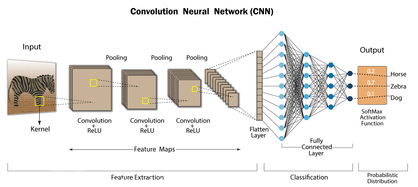
A simple ConvNet consists of a sequence of layers, each transforming the input volume into an output volume through a differentiable function. The main layers in ConvNet architectures are the Convolutional Layer, Pooling Layer, and Fully-Connected Layer, similar to those in regular Neural Networks. These layers are stacked to form a complete ConvNet architecture.
Example Architecture
For CIFAR-10 classification, a simple ConvNet could have the architecture [INPUT – CONV – RELU – POOL – FC]. Here’s a brief breakdown:
- INPUT [32x32x3]: Holds the raw pixel values of the image (width 32, height 32, 3 color channels).
- CONV Layer: Computes output of neurons connected to local regions in the input. Using 12 filters might result in a volume of [32x32x12].
- RELU Layer: Applies an elementwise activation function like max(0,x), keeping the volume size unchanged ([32x32x12]).
- POOL Layer: Performs downsampling along spatial dimensions, reducing the volume size to [16x16x12].
- FC Layer: Computes class scores, resulting in a volume of [1x1x10], with each number corresponding to a class score in CIFAR-10.
ConvNets transform the input image layer by layer from raw pixel values to final class scores. Some layers, like CONV and FC, contain parameters (weights and biases) that are trained using gradient descent, while others, like RELU and POOL, perform fixed functions without parameters.
Convolutional Layer
The Convolutional Layer (Conv Layer) is the core building block of Convolutional Networks, handling most of the computational load. It consists of a set of learnable filters that are small spatially (along width and height) but extend through the full depth of the input volume. For instance, a filter in the first layer of a ConvNet might be 5x5x3 (covering 5×5 pixels and all 3 color channels).
During the forward pass, each filter slides (convolves) across the input volume’s width and height, computing dot products between the filter’s weights and the input at each position. This process creates a 2D activation map representing the filter’s response at each spatial location. Multiple filters in each Conv Layer result in multiple activation maps, which are stacked to form the output volume.
Local Connectivity
Instead of connecting each neuron to all neurons in the previous layer (as in regular Neural Networks), Conv Layers connect each neuron to only a local region of the input volume. This local region is called the receptive field or filter size.
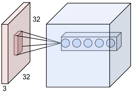
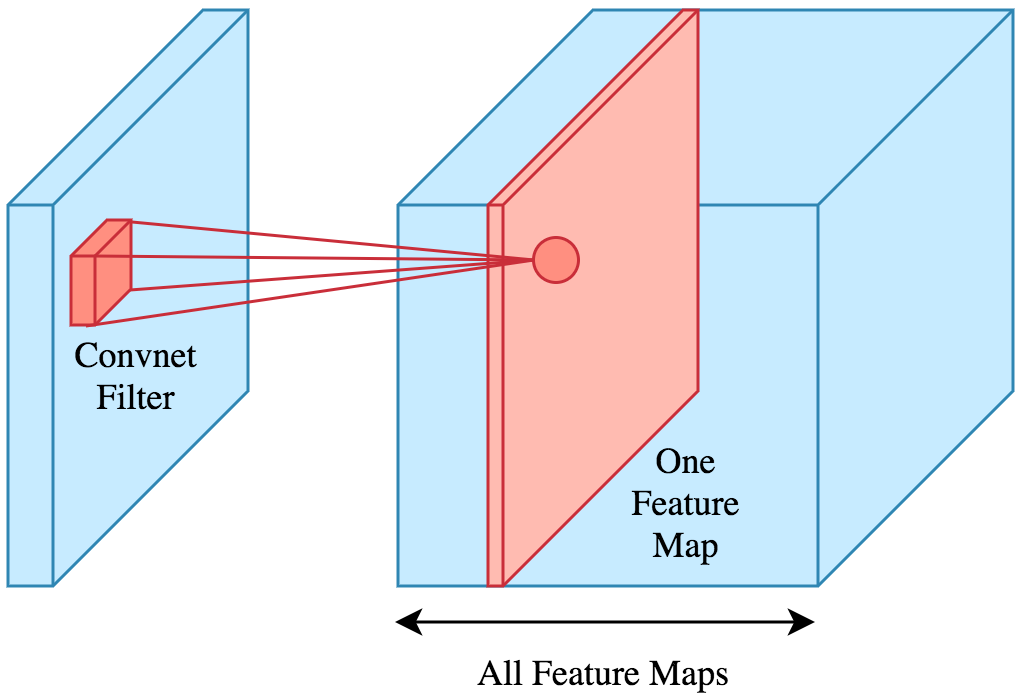
The image above illustrates this concept. The input volume on the left is a 32x32x3 image. The highlighted region shows a small local region (e.g., 5x5x3 region resulting in 75 weights and 1 bias) that a neuron in the Conv Layer connects to. This local connectivity allows each neuron to focus on a small part of the input, making the network more efficient.
The image illustrates how convolutional layers process input volumes. Here’s how it works:
- Input Volume: The left part of the image shows a 32x32x3 input volume (let’s say an image from the CIFAR-10 dataset).
- Local Region Connectivity: The highlighted patch in the input volume (5x5x3 region) represents the local connectivity of a neuron in the Conv Layer. Each neuron connects only to a small local region rather than the entire input volume.
- Output Volume: The right part of the image depicts the output volume produced by the Conv Layer. This volume is a stack of 2D activation maps generated by different filters.
Filters and Depth Slices
- Different Filters: Neurons at different depths of the output volume use different filters. For example, if the Conv Layer has 12 filters, there will be 12 different sets of weights and biases, each producing a separate 2D activation map.
- Same Filter in Depth Slice: Neurons within the same depth slice share the same filter weights and biases. This means that as the filter convolves across the input volume, it applies the same set of weights at each spatial location, ensuring consistent detection of features across the input.
Parameter Efficiency
Consider an input volume of 32x32x3 and a fully connected layer. If the next layer has 1,000 neurons, each of those neurons would need to connect to every pixel in the input volume. The total number of connections (or parameters) required would be:
- For each neuron: 32 (width) * 32 (height) * 3 (color channels) = 3,072 weights.
- For 1,000 neurons: 3,072 weights * 1,000 neurons = 3,072,000 weights.
- Additionally, each neuron has one bias term: 1,000 biases.
- The total number of parameters: 3,072,000 weights + 1,000 biases = 3,073,000 parameters.
If we increase the number of neurons in the fully connected layer to 10,000, the total number of parameters becomes:
- For each neuron: 32 (width) * 32 (height) * 3 (color channels) = 3,072 weights.
- For 10,000 neurons: 3,072 weights * 10,000 neurons + 10,000 biases = 30,730,000 parameters.
Now consider a Conv Layer with 12 filters of size 5×5 applied to the same input volume:
- Each filter has 5 (width) * 5 (height) * 3 (color channels) = 75 weights.
- For 12 filters: 75 weights * 12 filters = 900 weights.
- Additionally, each filter has one bias term: 12 biases.
- The total number of parameters: 900 weights + 12 biases = 912 parameters.
This demonstrates that a Conv Layer with 12 filters requires only 912 parameters, which is significantly fewer than the 30 million parameters required for a fully connected layer with 10,000 neurons.
Spatial Arrangement
Three hyperparameters control the Conv Layer’s output volume size: depth, stride, and zero-padding:
- Depth: The depth of the output volume is the number of filters used.
- Stride: The step size with which the filters slide over the input volume.
- Zero-padding: Padding added around the input volume’s border to control the spatial size of the output volume.
For example, let’s consider an input size of 32 by 32, a filter size of 5, a stride of 1, and zero-padding of 2. To compute the spatial size of the output volume, we can use the formula:
Output Size = (W – F + 2P) / S + 1
where:
– W is the input volume size,
– F is the receptive field size (filter size),
– S is the stride,
– P is the amount of zero padding.
Plugging in the values:
Output Size = (32 – 5 + 2 * 2) / 1 + 1
Output Size = (32 – 5 + 4) / 1 + 1
Output Size = 31 / 1 + 1
Output Size = 32
So, with an input size of 32 by 32, a filter size of 5, a stride of 1, and zero-padding of 2, the output size remains 32 by 32.
Using this formula, you can easily compute the output volume size for different configurations of input size, filter size, stride, and padding.
Parameter Sharing
Conv Layers use parameter sharing to control the number of parameters. Instead of each neuron having its own set of weights, neurons within the same depth slice share weights.
Notice that the parameter sharing assumption is relatively reasonable: If detecting a horizontal edge is important at some location in the image, it should intuitively be useful at some other location as well due to the translationally-invariant structure of images. This dramatically reduces the number of parameters, ensuring computational efficiency. For example, a Conv Layer with 96 filters of size 11x11x3 results in 34,944 parameters (96*(11*11*3) + 96 biases).
Implementation as Matrix Multiplication. The convolution operation in a Conv layer can be optimized using matrix multiplication. Local regions of the input image are stretched into columns, forming a matrix where each column represents a receptive field. Similarly, the filter weights are stretched into rows, forming another matrix where each row represents a filter. Multiplying these two matrices (using np.dot) efficiently performs the convolution. The resulting matrix is then reshaped back to its proper output dimensions. This method leverages efficient matrix multiplication libraries but uses more memory.
Pooling Layer
A Pooling layer is commonly inserted between Conv layers in a ConvNet to reduce the spatial size of the representation, thereby decreasing the number of parameters and computation in the network, which helps control overfitting.
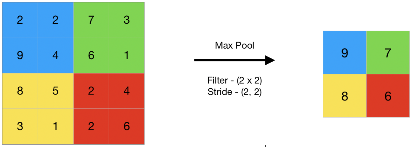
It operates independently on each depth slice of the input using the MAX operation, typically with filters of size 2×2 and a stride of 2, which reduces the input size by half along each spatial dimension. For example, a 224x224x64 input volume becomes 112x112x64 after pooling.
General Pooling
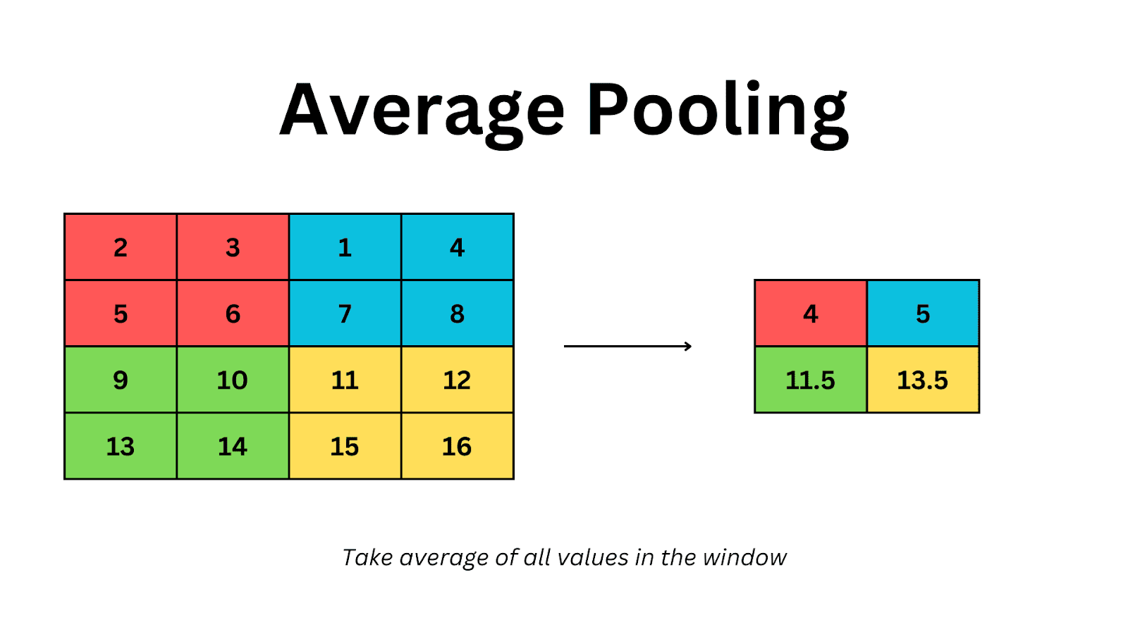
While max pooling is most common, pooling can also be done using average pooling or L2-norm pooling. Max pooling has been found to be more effective in practice.
Backpropagation in Pooling Layers
During backpropagation, only the gradient of the maximum value is routed back, which simplifies the gradient computation.
Getting Rid of Pooling
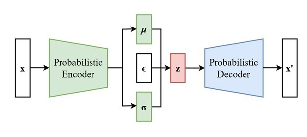
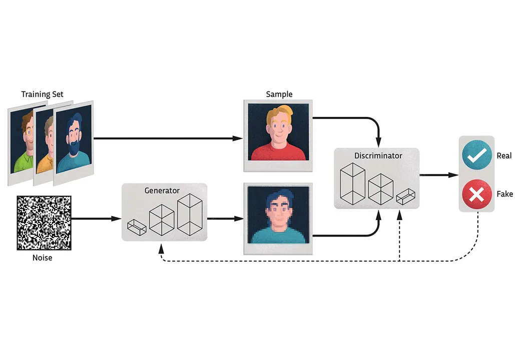
Some modern architectures propose eliminating pooling layers in favor of using Conv layers with larger strides to reduce the representation size. This approach has shown benefits in training certain models like VAEs and GANs.
Normalization Layer
Normalization layers, designed to mimic biological inhibition schemes, have largely fallen out of favor due to their minimal practical impact.
Fully-Connected Layer
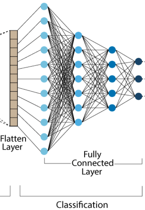
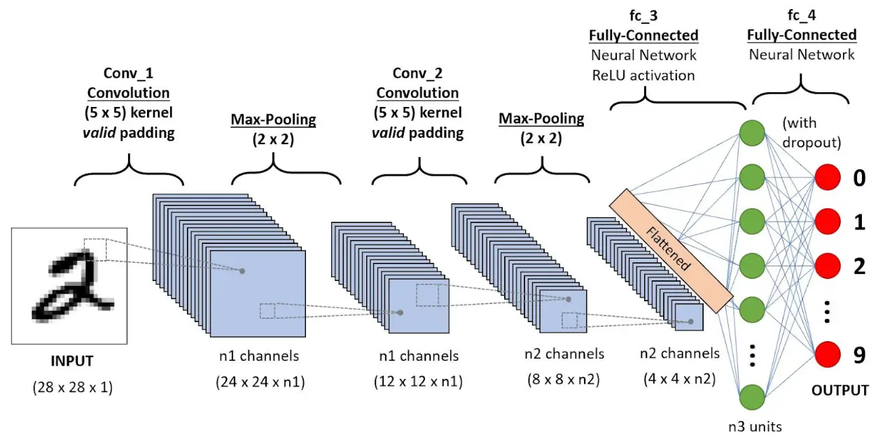
In a fully connected layer, each neuron connects to all activations from the previous layer. Their activations are computed through matrix multiplication followed by a bias offset, similar to traditional neural networks. Before a fully connected layer can process the activations, it’s often necessary to flatten the output of the previous layer, especially if it’s a convolutional layer. A flatten layer converts the multi-dimensional output of the convolutional layer into a one-dimensional vector, making it compatible for the subsequent fully connected layer. This transformation ensures that every activation can be connected to each neuron in the fully connected layer, maintaining the dense connectivity required for further processing and learning.
ConvNet Architectures
ConvNets typically consist of three main layer types: Convolutional (CONV), Pooling (POOL), and Fully-Connected (FC) layers. These layers are stacked together to form a complete ConvNet.
Layer Patterns
ConvNet architectures usually follow this pattern:
INPUT -> [[CONV -> RELU]*N -> POOL?]*M -> [FC -> RELU]*K -> FC
Where:
- N is the number of CONV -> RELU layers before an optional POOL layer.
- M is the number of such groups.
- K is the number of FC -> RELU layers.
Examples:
- Simple linear classifier: INPUT -> FC
- Basic ConvNet: INPUT -> CONV -> RELU -> FC
- Common ConvNet: INPUT -> [CONV -> RELU -> POOL]*2 -> FC -> RELU -> FC
- Deeper ConvNet: INPUT -> [CONV -> RELU -> CONV -> RELU -> POOL]*3 -> [FC -> RELU]*2 -> FC
Layer Sizing Patterns
- Input Size: The input layer should be divisible by 2 multiple times, e.g., 32, 64, 96, 224, 384, 512.
- Conv Layers: Use small filters (3×3 or 5×5) with stride 1 and appropriate padding to preserve spatial dimensions.
- Pooling Layers: Commonly use max-pooling with 2×2 receptive fields and stride 2 to downsample the spatial dimensions.
Case Studies of CNN Architectures
LeNet
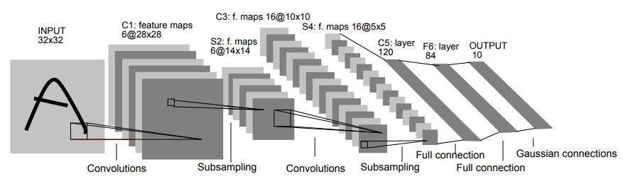
- Developed by Yann LeCun in the 1990s for digit recognition.
- Key in pioneering the use of ConvNets for practical applications like reading zip codes.
AlexNet
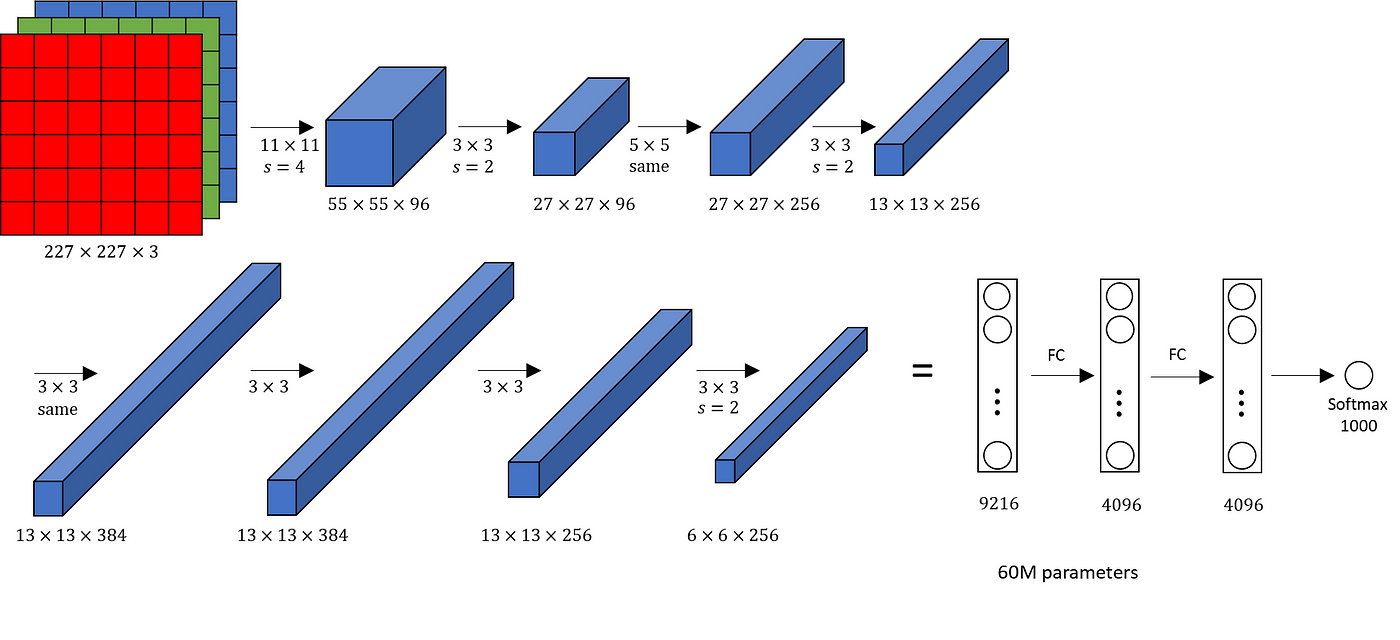
- Created by Alex Krizhevsky, Ilya Sutskever, and Geoff Hinton.
- Won the ImageNet ILSVRC challenge in 2012, outperforming the runner-up significantly.
- Introduced deeper and wider ConvNet structures with stacked CONV layers.
ZFNet
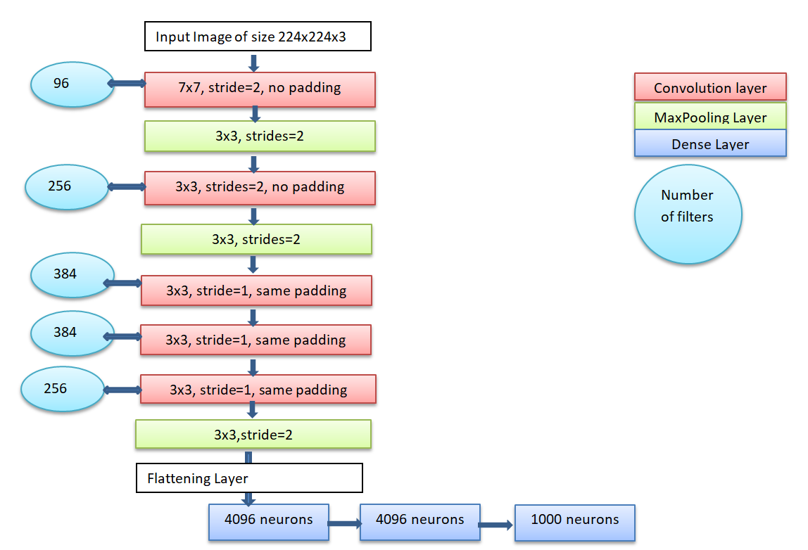
- Developed by Matthew Zeiler and Rob Fergus.
- Won ILSVRC 2013.
- Improved on AlexNet by tweaking hyperparameters, particularly in the middle convolutional layers.
GoogLeNet
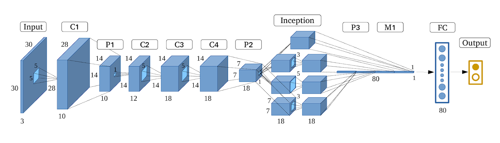
- Developed by Szegedy et al. from Google.
- Won ILSVRC 2014.
- Introduced the Inception module to reduce the number of parameters significantly.
- Replaced fully connected layers with average pooling at the top of the network.
VGGNet
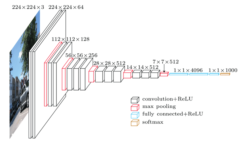
- Developed by Karen Simonyan and Andrew Zisserman.
- Runner-up in ILSVRC 2014.
- Demonstrated the importance of depth in ConvNets, with a simple and homogeneous architecture using 3×3 convolutions throughout.
- Despite high memory and parameter requirements, it showed excellent performance.
ResNet
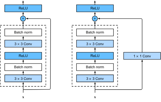
- Developed by Kaiming He et al.
- Won ILSVRC 2015.
- Introduced skip connections and heavy use of batch normalization.
- These skip connections enable the direct flow of information, like features, from earlier layers to later layers, also aiding in preserving gradients and promoting better convergence. This helps mitigate the vanishing gradient problem, where gradients become extremely small as they’re propagated backwards through many layers. With skip connections, gradients can flow directly through these shortcuts, allowing for better gradient flow during backpropagation.
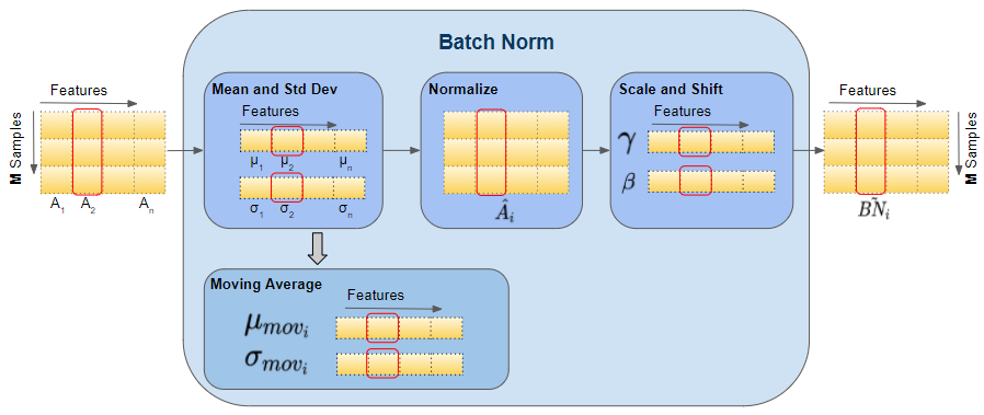
- Batch normalization normalizes the inputs of each layer by adjusting and scaling the activations. It helps prevent internal covariate shift, where the distribution of each layer’s inputs changes during training. This technique not only prevents vanishing or exploding gradients but also allows for higher learning rates and reduces the dependence on careful parameter initialization.
- Eliminated fully connected layers at the end of the network.
- Set a new standard for ConvNet performance and has become the default choice for many applications.
These case studies highlight the evolution and improvements in ConvNet architectures, each building on previous innovations to achieve better performance and efficiency.
Practical Advice
In most applications, use pretrained models from ImageNet and fine-tune them for your data rather than designing or training a ConvNet from scratch. This is called transfer learning and we’ll talk about it again near the end of the post.
Memory Considerations
When designing ConvNets, be aware of the memory constraints, especially the sizes of intermediate volumes, parameters, and additional data like batches. To estimate memory usage:
- Calculate the number of values in activations and gradients.
- Multiply by 4 bytes (for floating point) or 8 bytes (for double precision).
- Convert to GB by dividing by 1024 multiple times.
Reducing the batch size can help fit the network into available memory.
Visualizing What ConvNets Learn
Several techniques have been developed to understand and visualize the features learned by Convolutional Networks, addressing the criticism that neural network features are not interpretable.
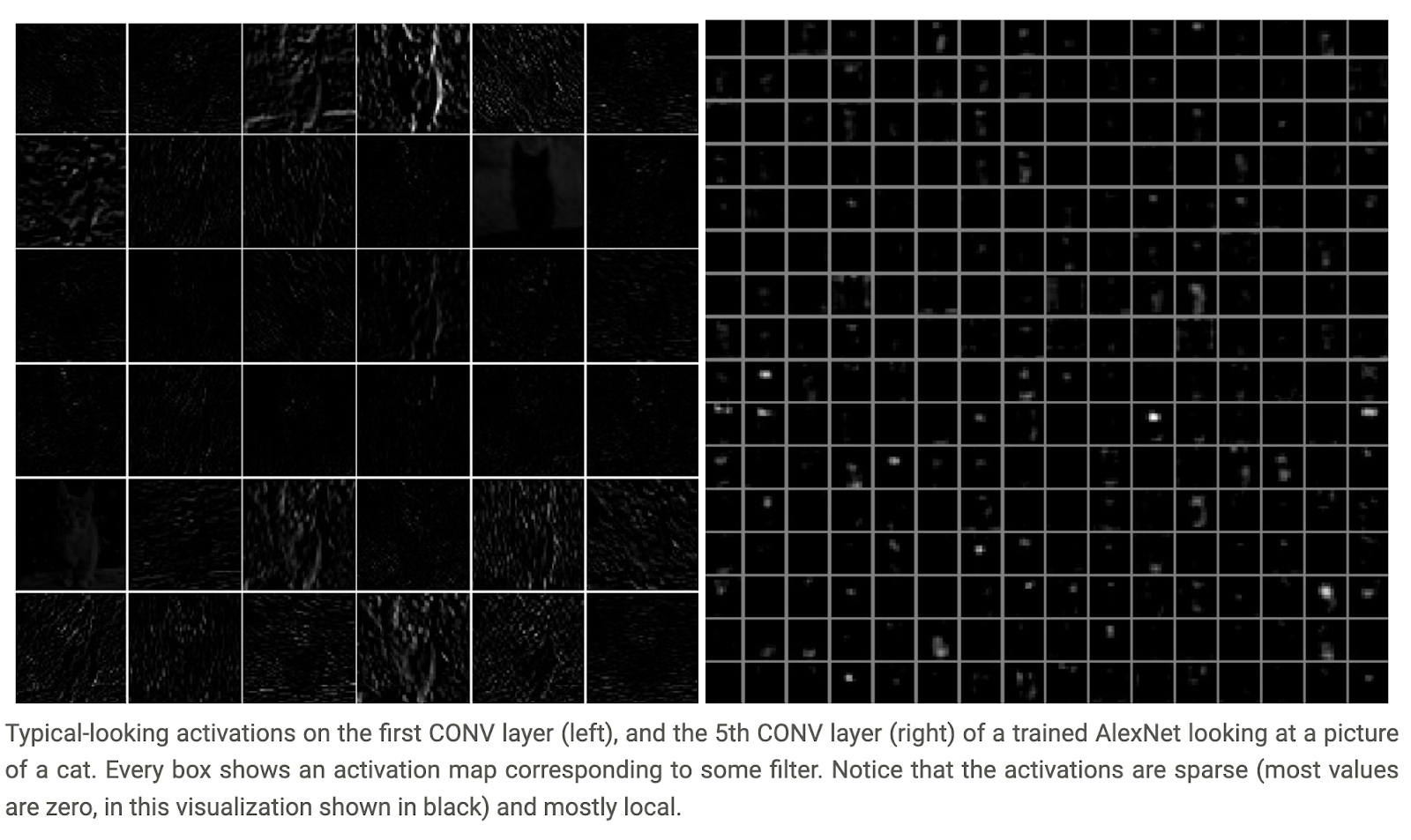
- Layer Activations
- Visualize network activations during the forward pass.
- Early activations are dense and blobby, becoming sparser and more localized as training progresses.
- Can reveal “dead filters” if activation maps are consistently zero.
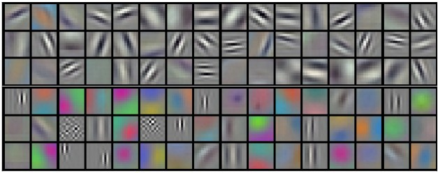
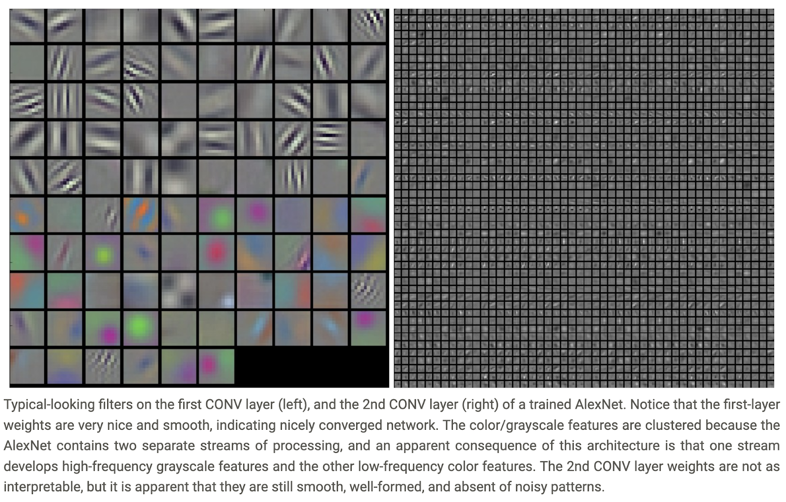
- Visualizing Weights
- Particularly effective for the first CONV layer.
- Well-trained networks show smooth, organized filters.
- Noisy patterns indicate insufficient training or overfitting.
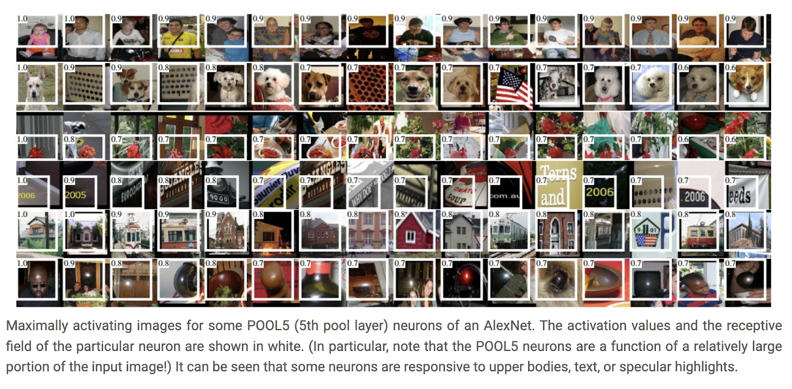
- Maximally Activating Images
- Identify images that activate a specific neuron the most.
- Helps understand what features a neuron detects.
- Not all neurons have clear semantic meanings; they represent basis vectors in the image patch space.
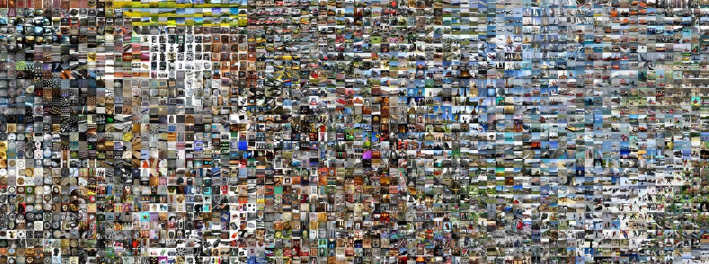
- t-SNE Embeddings
- Project high-dimensional CNN codes into 2D using t-SNE.
- Visualizes the similarity between images in the representation space.
- Similar images are placed near each other based on class and semantic features.
- Occluding Parts of the Image
- Determine which parts of the image contribute to the classification.
- Slide an occluder over the image and plot the class probability.
- Visualize as a heatmap showing the importance of different image regions.
These techniques provide insights into how ConvNets process and understand visual information, making the learned features more interpretable.
Transfer Learning
In practice, training an entire Convolutional Network from scratch is uncommon due to the large dataset size required. Instead, pretraining a ConvNet on a large dataset like ImageNet and using it for new tasks is more practical. There are three main strategies:
- ConvNet as Fixed Feature Extractor:
- Pretrain a ConvNet on ImageNet.
- Remove the last fully-connected layer.
- Use the remaining ConvNet as a fixed feature extractor for the new dataset, producing CNN codes (e.g., 4096-D vectors in AlexNet).
- Train a linear classifier (e.g., SVM or Softmax) on these features.
- Fine-tuning the ConvNet:
- Replace and retrain the classifier on top of the ConvNet.
- Optionally fine-tune the weights of the entire ConvNet or just the higher layers.
- Early layers contain generic features; later layers are more specific to the original dataset.
- Pretrained Models:
- Use pretrained ConvNet models available from resources like Caffe’s Model Zoo.
- Fine-tune these models for specific tasks.
When and How to Fine-Tune
Deciding the transfer learning approach depends on the size and similarity of the new dataset to the original dataset:
- Small and Similar Dataset:
- Use a linear classifier on CNN codes to avoid overfitting.
- Large and Similar Dataset:
- Fine-tune the entire network.
- Small and Different Dataset:
- Train a linear classifier, potentially from earlier layer activations to capture more generic features.
- Large and Different Dataset:
- Fine-tune the entire network or train from scratch, starting with pretrained weights.
Practical Tips
- Architecture Constraints: When using pretrained networks, you may be limited in modifying the architecture but can handle different spatial sizes due to parameter sharing.
- Learning Rates: Use a smaller learning rate for fine-tuning ConvNet weights compared to training the new linear classifier to avoid distorting pretrained weights too quickly.
These strategies and tips make transfer learning a powerful approach, leveraging pretrained ConvNets to achieve high performance on new tasks with limited data and computational resources.
In conclusion, Convolutional Neural Networks (CNNs) have revolutionized deep learning, particularly in computer vision, by efficiently processing and analyzing visual data. Throughout this post, we’ve explored CNN architecture, key layers, and practical applications, showcasing their unparalleled ability to recognize patterns and structures in images. While CNNs remain foundational, transformers are increasingly being used for visual tasks, offering exciting new possibilities. If you have any questions, leave a comment below. Like the post if you appreciated it, and subscribe to stay tuned for future posts, including an upcoming one on transformers. Thank you for reading!

I absolutely love your website.. Great colors & theme. Did you build this website yourself? Please reply back as I’m planning to create my own personal blog and want to learn where you got this from or just what the theme is called. Thank you!
Thanks! Yes, I built it myself and the theme is called Astra.