Tensors: The Building Blocks of Modern Machine Learning
Code and Notebook: https://github.com/Lumos-Academy/educational/blob/main/tensors/tensors.ipynb
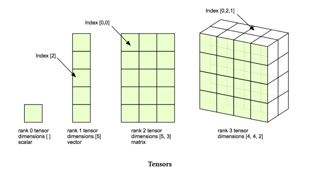
Tensors are fundamental mathematical objects used in various fields, including physics, engineering, and machine learning. In simple terms, a tensor is a generalization of vectors and matrices to potentially higher dimensions. They’re especially important in deep learning, where they represent the core data structure for neural networks.
Let’s break down the concept of tensors by dimension:
- Scalar (0-D Tensor):
A scalar is a single number. In tensor terms, it’s a 0-dimensional tensor.
# Scalar (0-D Tensor)
import numpy as np

scalar = np.array(5)
print(scalar)
print("Shape:", scalar.shape)
- Vector (1-D Tensor):
A vector is a 1-dimensional array of numbers.
# Vector (1-D Tensor)
vector = np.array([1, 2, 3, 4, 5])
print(vector)
print("Shape:", vector.shape)
- Matrix (2-D Tensor):
A matrix is a 2-dimensional array of numbers.
# Matrix (2-D Tensor)
matrix = np.array([[1, 2, 3],
                   [4, 5, 6],
                   [7, 8, 9]])
print(matrix)
print("Shape:", matrix.shape)
- Higher-Dimensional Tensors:
Tensors can have more than two dimensions. For example, a 3-D tensor could represent a cube of numbers.
# 3-D Tensor
tensor_3d = np.array([[[1, 2], [3, 4]],
                      [[5, 6], [7, 8]],
                      [[9, 10], [11, 12]]])
print(tensor_3d)
print("Shape:", tensor_3d.shape)
Tensors in Machine Learning:
In machine learning, tensors are used to represent various types of data:
- Input data (e.g., images, text)
- Model parameters (weights and biases)
- Intermediate representations in neural networks
Let’s create a simple example using PyTorch to demonstrate how tensors are used in a basic neural network:
import torch
import torch.nn as nn

# Create a random input tensor (batch_size, input_features)
input_tensor = torch.randn(32, 10)

# Define a simple neural network
class SimpleNN(nn.Module):
    def __init__(self):
        super(SimpleNN, self).__init__()
        self.fc1 = nn.Linear(10, 5)
        self.fc2 = nn.Linear(5, 1)

    def forward(self, x):
        x = torch.relu(self.fc1(x))
        x = self.fc2(x)
        return x

# Create an instance of the model
model = SimpleNN()

# Pass the input tensor through the model
output = model(input_tensor)

print("Input shape:", input_tensor.shape)
print("Output shape:", output.shape)
In this example, we create a random input tensor with 32 samples and 10 features each. We then define a simple neural network with two linear layers and pass the input through it. The shapes of the tensors change as they flow through the network.
Understanding tensor operations is crucial for working with neural networks and other machine learning models.
Common operations include:
- Reshaping
- Element-wise operations
- Matrix multiplication
- Reduction operations (sum, mean, etc.)
Here’s a quick example of some tensor operations:
import torch

# Create a tensor
a = torch.tensor([[1, 2], [3, 4]])

# Reshaping
b = a.reshape(4)
print("Reshaped:", b)

# Element-wise operation
c = a * 2
print("Element-wise multiplication:", c)

# Matrix multiplication
d = torch.matmul(a, a)
print("Matrix multiplication:", d)

# Reduction
e = torch.sum(a)
print("Sum of all elements:", e)
Tensors with Gradient Information
In addition to storing data, tensors in deep learning frameworks like PyTorch can also track gradient information. This capability is crucial for implementing backpropagation, the algorithm used to train neural networks.
When a tensor is created with requires_grad=True, it tells the framework to track operations performed on this tensor and compute gradients with respect to it. This is particularly useful for model parameters (weights and biases) and input tensors that require gradient computation.
Let’s demonstrate this with a PyTorch example:
import torch

# Create a tensor with gradient tracking
x = torch.tensor([[1., 2.], [3., 4.]], requires_grad=True)
print("x:", x)
print("x.requires_grad:", x.requires_grad)

# Perform some operations
y = x.pow(2).sum()
print("y:", y)

# Compute gradients
y.backward()

# Access the gradients
print("x.grad:", x.grad)
In this example:
- We create a tensor
xwithrequires_grad=True. - We perform operations on
xto createy. - We call
y.backward()to compute gradients. - The gradients are stored in
x.grad.
The x.grad tensor will contain the partial derivatives of y with respect to each element in x. This is the essence of automatic differentiation, which is key to training neural networks.
Let’s expand on this with a more practical example involving a simple neural network:
import torch
import torch.nn as nn

# Create a simple dataset
X = torch.tensor([[1.0, 2.0], [3.0, 4.0], [5.0, 6.0]], requires_grad=True)
y = torch.tensor([[3.0], [7.0], [11.0]])

# Define a simple neural network
class SimpleNN(nn.Module):
    def __init__(self):
        super(SimpleNN, self).__init__()
        self.linear = nn.Linear(2, 1)

    def forward(self, x):
        return self.linear(x)

# Create model, loss function, and optimizer
model = SimpleNN()
criterion = nn.MSELoss()
optimizer = torch.optim.SGD(model.parameters(), lr=0.01)

# Training loop
for epoch in range(100):
    # Forward pass
    y_pred = model(X)
    loss = criterion(y_pred, y)

    # Backward pass and optimization
    optimizer.zero_grad()
    loss.backward()
    optimizer.step()

    if (epoch + 1) % 10 == 0:
        print(f'Epoch [{epoch+1}/100], Loss: {loss.item():.4f}')

# Print model parameters and their gradients
for name, param in model.named_parameters():
    print(f"{name}:")
    print("  Parameter:", param.data)
    print("  Gradient:", param.grad)

# Make a prediction with gradient tracking
X_test = torch.tensor([[2.0, 3.0]], requires_grad=True)
y_pred = model(X_test)
y_pred.backward()

print("\nGradient of input:")
print(X_test.grad)
This example demonstrates several important concepts:
- We create an input tensor X with requires_grad=True to track gradients through the entire computation graph.
- The model parameters (weights and biases of the linear layer) automatically have requires_grad=True.
- During training, we compute the loss and call loss.backward() to compute gradients for all tensors in the computation graph that require gradients.
- The optimizer uses these gradients to update the model parameters.
- After training, we can inspect the gradients of the model parameters.
- We can also compute gradients with respect to input tensors, as shown with X_test.
Understanding how tensors track gradient information is crucial for:
- Implementing custom neural network layers
- Debugging backpropagation issues
- Implementing advanced optimization techniques
- Analyzing model sensitivity to inputs
This gradient-tracking capability of tensors, combined with automatic differentiation, is what makes modern deep learning frameworks so powerful and easy to use.
In conclusion, tensors are versatile mathematical objects that form the foundation of modern machine learning. They can represent data of various dimensions, from scalars to complex multi-dimensional arrays. In deep learning frameworks, tensors not only store data but also track gradient information, enabling efficient training of neural networks through backpropagation. Understanding tensors and their operations is essential for anyone working in the field of machine learning and artificial intelligence.